Michael Song's Projects
Animation of Projectile Motion with and without Air Resistance
Project duration
June, 2021
Introduction
Projectiles are very common in our daily life, such as throwing a water-balloon, shooting a basketball, shot put, etc. From my AP physics class, I learned that the motion of projectiles has a parabolic trajectory when air resistance is negligible, but we never explored the scenario containing air resistance. This project demonstrates the effect of air resistance on the motion of projectiles through the visualizations of 2-d projectiles in Python. Click here to jump to see the animation result.
Click here to jump to see the animation result.
Objectives
The objectives of this projects include • To animate the motion of projectiles with and without considering air resistance. • To compute and compare instantaneous locations, velocities, travel distances and energies.
Methods
1. Physics and Math
It is well known that air resistance depends on the speed, shape and size of projectiles, density of air, and some other factors. Therefore, it can be a complex phenomenon to study and measure. In this project, we simplify the model by assuming that the drag force of air resistance is proportional to the speed of the projectile and always opposite to the direction of its velocity
where \(k\) is a positive constant describing the air resistance coefficient. By ignoring non-linear components, this approximation might not be very accurate in reality, but it allows separating the drag force into horizontal and vertical directions, respectively, and makes differential equations easy to solve.
Consider a projectile of mass \(m\), initial position, \(\left( { {x_0},{y_0} } \right)\), initial velocity, \({\vec v_0} = \left( { {v_{x,0} },{v_{y,0} } } \right)\) and initial launch angle, \(\theta \) (Figure 1).
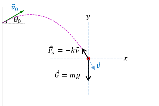
Figure 1 Illustration of the projectile.
The \(x\)- and \(y\)-components of initial velocity is
\({v_{x,0}} = {v_0}\cos \theta \)
\({v_{y,0}} = {v_0}\sin \theta \)
(2)Using the linear model of air resistance (Eq. 1) and Newton’s 2nd law:
\(m\frac{ {d{v_x} } }{ {dt} } = - k{v_x}\)
\(m\frac{ {d{v_y} } }{ {dt} } = - mg - k{v_y}\)
(3)Solving these differential equations with the initial conditions, gives the instantaneous velocity as a function of time \(t\)
\({v_x}\left( t \right) = {v_{x,0} } \cdot {e^{ - \frac{ {kt}}{m} } }\)
\({v_y}\left( t \right) = {v_{y,0} } \cdot {e^{ - \frac{ {kt} }{m} } } + \frac{ {mg} }{k}\left( { {e^{ - \frac{ {kt} }{m} } } - 1} \right)\)
(4)Integrating \({v_x}\left( t \right)\) and \({v_y}\left( t \right)\) with respect to \(t\) gives instantaneous positions
\(x\left( t \right) = {x_0} + {v_{x,0}} \times \frac{m}{k}\left( {1 - {e^{ - \frac{ {kt} }{m} } } } \right)\)
\(y\left( t \right) = {y_0} + {v_{y,0}} \times \frac{m}{k}\left( {1 - {e^{ - \frac{ {kt} }{m} } } } \right) + \frac{ { {m^2}g} }{ { {k^2} } }\left( {1 - \frac{k}{m}t - {e^{ - \frac{ {kt} }{m} } } } \right)\)
(5)The above equations are the general formulas for the linear model of air resistance. In the absence of air resistance, the formulas can be derived from Equation (3) by setting \(k = 0\) as below:
\(m\frac{ {d{v_x} } }{ {dt} } = 0\)
\(m\frac{ {d{v_y} } }{ {dt} } = -mg\)
(6)\({v_x}\left( t \right) = {v_{x,0} }\)
\({v_y}\left( t \right) = {v_{y,0} } - gt\)
(7)\(x\left( t \right) = {x_0} + {v_{x,0} } \times t\)
\(y\left( t \right) = {y_0} + {v_{y,0} } \times t + \frac{1}{2}g{t^2}\)
(8)In fact, as an alternative method, if you substitute the Taylor expansion \({e^{ - \frac{ {kt} }{m} } } = 1 - \frac{ {kt} }{m} + \frac{ { { {\left( {\frac{ {kt} }{m}} \right)}^2} } }{ {2!}} + \cdots \) into Equations (4) and (5) and take limit of \(k \to 0\), you will get the same results as Equations (7) and (8).
As for the accumulated travel distance \(d\left( { {t_n} } \right)\), it can computed by adding the new traveling length to the previous accumulated travel length
The kinetic, potential, and total mechanic energies can be computed using the instantaneous speed and positions, accordingly.
2. Computer programming
The animation part of this project was implemented using Python with the Matplotlib package. There are 4 major components:
-
In the global scope, the simulation parameters are specified, such as the initial position, velocity, launching angle, mass, air resistance coefficient, and the Gravitational Constant. The drawing and text objects are also created and will updated during animation.
-
The
init()function to reset the drawing and text objects, as well as the intermediate variables. -
The
animate(i)function to compute the instantaneous quantities on-the-fly and update the drawing and text objects. -
The
main()function callsanimation.FuncAnimation()from the Matplotlib package to create the animation, which repeatedly calls theanimate(i)function above to refresh the display. It also saves the animation to video files.
Results and Discussions
The animation video is shown below. The trajectories with and without air resistance are drawn in red and blue, respectively. Please click the Replay button to view the video.
We observed a few differences between the two scenarios.
- Due to the impact of air resistance, the projectile has a trajectory different from that in absence of air resistance, and it is no longer a parabolic curve.
- With air resistance, the projectile flies slower than that in absence of air resistance. At the same intervals of time, its speed (magnitude of velocity) and travel distance are lower and smaller.
- With air resistance, the projectile loses mechanical energy, which was used to overcome the resistance and converted to heat.
Summary
In this independent project, I explored the impact of air resistance on projectiles beyond what was covered in our AP physics classroom. This exploration involved in building a model based on Physics, solving differential equations using math, and making vivid animations using computer programming. The visualized results provide us a view and sense different from textbook. It is a fun and interesting project that anyone can do!